Project: || Prior Study | Task 1 | Task 2 | Task 3 | Task 4 | Task 5 | Tasks 6-7 | Deliverables | Home
The Miasma Beach Transportation Model
Task 3. DEMAND FORECASTING: TRIP GENERATION
The first two tasks have focused on the development of a network that represents the transportation system of Miasma Beach. Task 3 develops the specifications for the activity system of the region. Recall that the area has been divided into six Traffic Analysis Zones (1 through 6), with two external stations (7 and 8) that serve as control points with areas not directly part of the study area. The modeling approach is to calibrate and validate trip generation and trip distribution models for the six internal zones only. Interactions with the external area (via the external stations) have been modeled independently and these results will be provided in Task 5.
3.1 Description of the Zoning System
Figure 2 depicts the defined TAZs superimposed on the corrected Miasma Beach 2020 base transportation network (verify that all network edits (Tasks 1 and 2) have been made before proceeding).
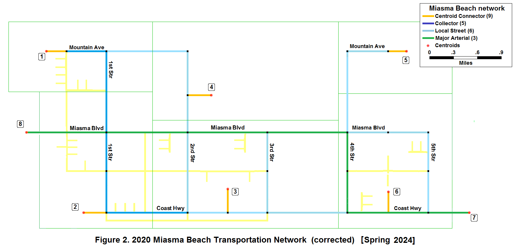
Zone 1 forms the Old Town Central Business District (CBD) and contain much of the total employment in the City. Zones 2 and 3 form a beachside community, a residential area with some retail activity along Coast Highway. Zone 4 is an agricultural area, with packing and processing industries, east of the CBD and north of Zone 3. Zones 5 and 6 are developing residential zones located east of the Miasma wetlands. Zone 6 is older and more developed than Zone 5. Similar to Zone 3, Zone 6 is oriented toward the beach. Zones 7 and 8 are External Stations: Zone 7 is at the eastern edge where Coast Highway heads toward the City of Miasma; Zone 8 is at western end of Miasma Blvd where SR-1 heads into the Miasma Mountains toward Port Miasma. A variety of demographic characteristics have been assembled for the six TAZs (data are provided in Table 2).
           Table 2. 2020 Miasma Beach Demographic Data
-----------------------------------------------------------------
 ZONE  POP  LABF  CARS  HINC    HH  EIND  ERET  EOTH  ETOT  AREA
-----------------------------------------------------------------
   1  3000  1100   900 29850   700   400   150  1000  1550  1.56
   2  1550  1300   600 44850   800   300   225  1300  1825  2.53
   3  3500  1200  2500 83100  1000     0   350   250   600  3.10
   4     0     0     0     0     0  1400   150   200  1750  2.83
   5  2450  1400  2000 49500   950     0   100    50   150  1.27
   6  5000  1800  2250 57000  1550     0   425   500   925  3.09
-----------------------------------------------------------------
 Tot 15500  6800  8250        5000  2100  1400  3300  6800 14.38
 Mean 2583  1133  1375 55050   833   350   233   550  1133  2.40
-----------------------------------------------------------------
 Note: Weighted mean used for income.

                Definition of Variables in Table 3
-------------------------------------------------------------------
 POP  = zone population               EIND = basic employment
 LABF = labor force (by residence)    ERET = retail employment
 CARS = total cars in zone            EOTH = other employment
 HINC = median zone household income  ETOT = total zone employment
 HH   = number of households in zone  Area = zone area (sq.mi.)
-------------------------------------------------------------------
Note: basic employment includes agricultural and industrial
3.2 Development of Trip Production and Attraction Models
As part of the development of the Miasma Beach Transportation Model, a formal home interview survey was conducted. Travel diaries were collected for all members of approximately 1000 households in the six internal zones. An extensive Cordon Survey also was conducted to develop estimates of traffic entering and exiting the area at the defined external stations (see Task 5). Preliminary analysis of survey data produced population-level estimates of trip productions and attractions for the study area. Total trips were segmented into Home Based Work (HBW), Home Based Other (HBO), and Non-Home Based (NHB) trips.
 Table 3. 2020 Miasma Beach Productions and Attractions
-------------------------------------------------------------
 ZONE TOT/P  TOT/A  HBW/P  HBW/A  HBO/P  HBO/A  NHB/P  NHB/A
-------------------------------------------------------------
   1  11550  10300   1800   3200   5500   4800   4250   2300
   2  11800  11800   1800   2800   5500   6000   4500   3000
   3  12050  12300   2700   1100   6600   6900   2750   4300
   4   1500   5600      0   3100      0   1800   1500    700
   5   8850   4800   2200    300   5400   1800   1250   2700
   6  14250  15200   3500   1500   7000   8700   3750   5000
-------------------------------------------------------------
 Tot  60000  60000  12000  12000  30000  30000  18000  18000
Mean  10000  10000   2000   2000   5000   5000   3000   3000
-------------------------------------------------------------
An estimate of 60,000 daily person trips were generated by Miasma Beach residents in the base year (2020); Table 3 presents base year trip productions and attractions. The estimated trips are split 20 percent HBW, 50 percent HBO, and 30 percent NHB. These trip types are fundamentally different based on such attributes as time-of-day, mean trip length, and vehicle occupancy.
The tabulated demographic and trip end data provided may be used to develop and/or apply zonal production and attraction trip generation models for Home-Based Work (HBW), Home-Based Other (HBO), and Non home-Based (NHB) trips.
3.2.1 Model Specification for Trip Generation
Production and attraction models have been estimated for some of the trip types
(these are summarized in Table 4a and 4b) but teams must estimate some models.
|
Spring 2024 Instructions: Each project Consulting Team will estimate and/or apply different combinations of the HBW, HBO, and NHB trip production models. Click HERE for instructions! |
It is recommended that you either verify the models provided using TransCAD or attempt to estimate alternative (perhaps better) production and attraction models. Provide a summary table of estimation results for all specified models as well as for any proposed alternative models. Be sure to include all model summary statistics.
  Table 4a. Estimated Trip Production Models [coef (t)]
 --------------------------------------------------------
  Variable    NHB#1     NHB#2       HBO#1     HBO#2
 --------------------------------------------------------
  HH          -         -           4.60      -
              -         -          (4.45)     -

  POP         0.32      0.21        -         1.29
             (3.87)    (2.33)       -        (3.51)

  ERET        -         2.15        -         -
              -        (1.81)       -         -

  EOTH        2.54      2.53        -         -
             (8.88)   (11.73)       -         -

  Const.    770.99    572.50     1169.51   1666.83
 --------------------------------------------------------
  Obser.      6         6           6         6
  R-sq        0.97      0.99        0.83      0.76
  F-ratio    46.85     56.23       19.77     12.33
 --------------------------------------------------------
  OLS coef (t-stat)

    Table 4b. Estimated Attraction Models [coef (t)]
 --------------------------------------------------------
  Variable       NHB                   HBO
 --------------------------------------------------------
  HH            2.09 (4.91)            -
  ERET          4.40 (2.64)          19.70 (8.36)
  EOTH                                2.01 (3.31)
  ETOT          -                     -
  Const.      233.22               -705.37
 --------------------------------------------------------
  Obser.        6                     6
  R-sq          0.97                  0.96
  F-ratio      46.48                 41.13
 --------------------------------------------------------
Team Assignments for TG Models (CEE123 and CEE223): Table 4c
3.2.2 Preparation of Input Data
The Miasma Beach trip production and attraction models will be estimated using
regression analysis, with the dependent variables being zonal productions and
attractions, respectively (from Table 3). Independent variables are demographic
variables (from Table 2). The demographic variables for each TAZ are included
in the TAZ Geographic file. Open the TAZ Geographic file and click the
New Dataview button to open the TAZ dataview. Sort by ascending
order of ID to compare the dataview with Table 2.
|
HELP: Productions and attractions are not included in the original TAZ file so these fields from Table 3 must be appended to the TAZ dataview. Click HERE for assistance!. |
3.2.3 Estimating HBW Trip Generation Models
Using 2020 Miasma Beach activity system data and the expanded trip data in
Tables 2 and 3, develop trip generation models for HBW productions and
attractions. Display these dependent and independent variables in the TAZ
dataview to begin the model estimation process. If previously estimated models
are being applied, then go to section 3.2.4.
CEE223 Teams must also estimate zonal rate models for HBO and NHB productions.
|
HELP: If you are estimating new models, utilize TransCAD's Model Estimation procedure. Click HERE for TransCAD assistance!. |
Follow the same procedure to estimate at least two potential models for HBW productions. You must estimate the production model identified in Table 4c; you must estimate the attraction model in Table 4c. Compare all estimated HBW models and determine which one is "best". As a rough guide, the final R-squared value should be 0.70 or better for the selected model. Tabulate ALL estimated HBW models and supporting statistics.
3.2.4 Create Model Files of HBO and NHB Productions and Attractions
Previously estimated trip generation models are summarized in Table 4a and 4b and
may be used to create TransCAD production and attraction model files (*.mod). The
task report should provide a table summarizing all models utilized, including all
summary statistics, whether new models or previously estimated models are utilized.
|
HELP: A Model File stores the variables and parameters of a TransCAD model. To create a file for an existing model, Click HERE for TransCAD assistance!. |
3.2.5 Applying Model Files of All Three Trip Purposes
Once model files are created for productions and attractions of all three
trip purposes, apply them to estimate trip ends for Miasma Beach.
|
HELP: To Apply a model file, select Planning / Trip Production / Apply a Model. Click HERE for TransCAD assistance! |
3.3 Trip Balancing
In trip generation, trip productions and trip attractions are estimated separately. The total number of trip productions, therefore, will typically not equal the total number of attractions. Any difference will violate the requirements for trip distribution analysis (and subsequent stages). The trip ends must be "balanced" so that the total number of productions equals the total number of attractions for each trip purpose (HBW, HBO, and NHB).
In practice, it is standard practice to hold trip productions constant, rather than attractions, when balancing trip ends. Trip productions are usually strongly related to zonal demographics, thus, the resulting production models are usually effective in replicating actual productions. On the other hand, there can be many factors that affect the number of trips attracted to a TAZ, thus, estimated attraction models often do not replicate attractions that well. For this reason, trip production estimates are typically considered more valid and thus are held constant. Conventionally, internal and external trip ends are combined prior to balancing. For Miasma Beach, external trips are already balanced, thus, only internal trips need be balanced at this point.
3.3.1 Balance (Normalize) Trip Attractions
Normalize zonal trip ends for HBW, HBO, and NHB trips for Miasma Beach,
holding productions constant (or providing justification for not doing so).
Tabulate productions with both initial and normalized attaractions
|
HELP: TransCAD provides a built-in procedure for trip balancing. With TAZ as the working layer, go to Planning / Balance. Click HERE for TransCAD assistance! |
3.3.2 Re-Allocate NHB Trip Attractions
While total NHB trip productions provide a reasonable estimate of total trips,
and thus serves as the normalization factor for total trip attractions, the
actual zone by zone distribution of (normalized) trip attractions provides a
better estimate of the zone-by-zone distribution of trip productions for NHB
trips. Re-allocate zonal NHB trip productions to be equal to zonal NHB
trip attractions.
3.3.3 Summary of Trip Production and Attraction Models
Provide a summary table comparing the estimated values of all three trip purposes.
Compute a "goodness-of-fit" measure to show how close the estimated
trip ends are to the "observed" values in Table 3.
3.4 Prepare Task 3 Documentation
Include all relevant layouts, outputs, and model files. Since each consultant uses a different set of generation models, final results will vary from those of other consultants. Include regression analysis results for all attempted models in an appendix. Follow Project Format Guidelines in the preparation of this report. This report will be submitted as part of Interim Report 2 with the results of Tasks 4 and 5.